This is a rough translation of the original portuguese version (chapters 1 and 2... only). Please use a compatible HTML-unicode Browser

Numerical representation

The current positional number notation was introduced in the Middle Ages by influence of Al-Kharizmi works (IX century), and allowed a considerable development of Calculus in Western Europe. The Hindu notion of zero generated a concept of representation that was absent in earlier millenia. The ease of calculations with this new representation has meant that the Greco-Roman cumulative notation was gradually abandoned ... nevertheless at a medieval rhythm. The choice of a basis still posed some problems for axiomatic medieval scholars. For example, the representation of 1/3 = 0.3333… could never be exact in decimal notation. If fractions (rational numbers) have a periodical decimal sequence, real numbers like √ 2= 1.414213562373… presented an unpredictable sequence of digits. Its decimal representation is always limited to a finite number of digits, and to a consequent error. It was only at the end of the XIX century, with G. Cantor, that real numbers were defined as (equivalence classes of) Cauchy sequences of rational numbers, where the sequence: x0=1, x1=1.4, x2=1.41, x3=1.414, x4=1.4142, ... is just a representative of all rational sequences that converge to the real number √ 2. This interpretation of Cantor represented a great conceptual advance, allowing further to distinguish countable infinity from continuous infinity. It is clear that the choice of the decimal basis for a real number representative is just the most common choice from an uncountable number of other possibilities. Already in the XVII century, Leibniz advocated advantages in binary representation − which is adopted nowadays in internal computer routines.   In general we can use any natural base β > 1, to write a real number. For instance, in Scientific Notation (usually β=10), x = ± (0. a1 a2 ... an ...)β × βt = ±   ∞ ∑ k=1 ak βt-k the digits ak ranging from 0 to β-1. To have uniqueness of exponent representation, a1≠ 0 and the zero is represented separately. This avoids several possibilities of representation as in 0.1 × β1 = 0.01 × β2 = 0.001 × β3 = 1 by choosing only the first. Note that, by convention, 0.999… is identified with the representation 1.000… (both sequences converge to 1).

Floating Point Representation

Unless you were in possession of a machine with infinite memory (... a theoretical Turing machine), the representation of a number must be finite. Thus we must consider a finite number of digits in the mantissa and a limitation of the exponents allowed.

Definition: Floating Point System The FP(β, n, t-, t+) system is the set of rational numbers FP(β, n, t-, t+) = {0} ∪ { ± 0. a1 a2 ... an × βt : ak∈ {0,..., β-1}, a1≠ 0, t∈ {t-, ..., t+ } }

Other Remarks: (i) Note that as a1 ≠ 0, zero must be represented separately (it might be a bit, a zero flag, as there is a bit that denotes the sign sign flag). (ii) Usually β=10, but binary representation β=2 is preferred in computers (the digits ai might be 0 or 1). Details on computer implementation may be found in the link IEEE 754-1985 . (iii) In programming languages (such as C, Fortran, Matlab) these FP systems are set when we declare the variables. Usually words like single, float, real*4,... stand for a single precision FP system with 4 bytes (23 bits − binary digits in the mantissa ~ up to 8 decimal digits). More recently it is standard to use double precision FP systems with 8 bytes (53 bits − binary digits in the mantissa ~ up to 16 decimal digits) and the variables are declared as double, float, real*8,...   Thus, we must map the real numbers to the rational number set FP, fl: R → FP(β, n, t-, t+) ⊂ Q and two type of limitations occur, leading to errors: Finite exponent limitations (errors that may abort execution): Overflow: when the exponent t is greater than t+. Underflow: when the exponent t is less than t-. Finite mantissa limitations (errors that we will study): Rounding errors: truncation and rounding.

Rounding

Given a real number, represented in scientific notation x = ± 0. a1 a2 ... an an+1 .... × βt while storing it in a system FP(β,n) we might be forced to suppress further digits in the mantissa. To proceed with that conversion we consider two types of rounding: Truncation flc(x) = ± 0. a1 a2 ... an × βt Rounding (half-up) (note: β > 2 is even) fls(x) = ± 0. a1' a2' ... an' × βt' The digits ak' coincide with ak and the exponent t' coincides with t, if an+1 < β/2. If an+1 > β/2 then the digits ai' and the exponent t' result from the representation of the sum 0. a1 a2 ... an × βt + βt − n. Remarks: (i) We may also consider fls(x) = flc(x +  1/2 βt − n) (ii) It should be noted that for statiscal purposes there is also a Round-to-even method that ensures a better distribution (in this method, the final rounding number should have an even mantissa − for instance, both 11.5 and 12.5 are rounded to the nearest even number 12).

Definition: Consider x an exact value and x~ an approximated value of x, we define: Error : ex( x~ ) = x − x~ Absolute error : |ex( x~ )| = |x − x~| Relative error (x ≠ 0): |δx( x~ )| with δx( x~ ) =   ex( x~ ) x - If there is no confusion with the approximation of x, we simply write ex to denote ex( x~ ), and likewise δx for the relative error. - We also use δx~ when it is more important to emphasize which is the approximation.

As in a FP system the rounding errors are inherent, we bound the rounding relative error |δarr(x)|, meaning δarr(x) = δx(fl(x)) =   x − fl(x) x

Theorem: For any x: fl(x)∈ FP(β, n), we have the relative error estimates: Truncation : |δarr(x) | < uc = β1-n Rounding : |δarr(x) | < us =  1/2 β1-n The bounds u are sometimes called rounding units.

proof: We prove for truncation. Consider any real number x x = ± 0.a1 ... an an+1 ... × βt As a1≠ 0 then a1≥ 1 and |x|≥ 0.1 × βt = βt − 1 On the other hand |earr| = |x − flc(x)| = |0.a1 ... an an+1... − 0.a1 ... an| × βt = 0.0 ... 0 an+1... × βt ≤ 0.0 ... 1 0 ... × βt = βt − n implies |δarr| = |earr|/|x| ≤ βt − n / βt − 1 = β1 − n (The proof for rounding is similar, and these estimates may be slightly improved...)

Remark Note that in a FP system we never round to zero. In some calculator machines, or in some ill implemented FP systems, it is common to see an overflow error, but not an underflow error, meaning that small absolute values are improperly rounded to zero. This leads to odd situations, like null values for exponentials... for instance, exp(-exp(8)) = 0.243… × 10-1294 may be zero in your calculator, without an "underflow warning". - How to present the result, using a conventional machine? In these cases you should separate calculations − what you need to compute from what is not representable. Thus, we may reduce to powers of 10, using logarithms, and presenting the result afterwards: e-exp(8) = 10-exp(8)/log(10) = 10-1294.6136 note that the operation -exp(8)/log(10) presents no problems for the calculator, and separating the decimal part of the exponent 10-0.6136=0.2434… we get the mantissa.   These type of errors may get worst while proceeding with further calculations... just note that if the result was 0 we could not get back the logarithm that should be -exp(8).

Error propagation in functions

Consider now the study of error propagation that results from applying a function or an operation to real numbers. Generally, we want to know if a function f does or does not affect much the proximity of the original values: x~ ≈ x ⇒ f(x~ ) ≈ f(x), in terms of the relative error. Applying Lagrange's Theorem, ef(x) = f(x) − f(x~ ) = f '(ξ) (x-x~) = f '(ξ)ex with ξ∈ [ x; x~ ], supposing that f∈ C1 (in the interval). It results (for x≠ 0, f(x)≠ 0) δf(x) = ef(x)/f(x) =   f '(ξ) f(x) ex =   x f '(ξ) f(x) δx and we may get the estimate for the relative error: |δf(x) | ≤   |x| maxξ∈ [x,x~] |f '(ξ)| |f(x)| |δx| . This estimate is not very useful, and it is more simple to consider the approximation ξ≈ x, which is a 1st order (or linear) approximation, in terms of the Taylor expansion. In fact, neglecting the term o(ex) in f(x~ ) = f(x) + f '(x)ex + o(ex) we get ef(x)≈ f '(x)ex, and dividing by f(x), we again get the approximation δf(x) ≈   x f '(x) f(x) δx which allows us to evaluate the error propagation from a function.

Definition: The value Pf(x) = x f '(x)/f(x) is called the condition number of f in x, and we have δf(x) ≈ Pf(x) δx

If |Pf(x)| is large this means that the relative error is considerably increased through the application of the function f. On the other hand if it is small, this means that you may get a relatively good approximation of f(x) even with considerable errors in x.

Examples: If f(x)=xp, we get Pf(x)=p, and therefore δx^p ≈ p δx. We conclude that for larger powers the initial relative error will be quite increased. If f(x)=ex, we get Pf(x)=x, thus δexp(x) ≈ x δx. We conclude that for large |x| elevado, the initial relative error will be quite increased. If f(x)=x-a, (a ≠ 0, constant) we get Pf(x)=x/(x-a), and therefore δx-a = x/(x-a) δx. We conclude that for x ≈ a, the initial relative error will be largely increased. This example shows that the sum/subtraction may lead to significative perturbations on the calculations, due to} "subtractive cancellation". If f(x)=ax, (a ≠ 0, constant) we get Pf(x)=1, and therefore δax = δx. In this case the original error is not affected. As counterpart to some of the previous examples, the propagation may lead to advantageous situations ... while evaluating xp if p ≈ 0 (root extraction), the relative error decreases, and the same happens for ex or x-a when x≈ 0. In these cases, a reasonable approximation of x may lead to an excellent result in terms of f(x).

Definition: We say that a function f is ill conditioned near a point z if, in the limit, |Pf(z)| = ∞.

Operations (functions with two or more variables) In the case of two (or several) variables, we must consider simultaneous errors in both variables. Considering the Taylor expansion with two variables (∂m represents the partial derivative in the m-th variable): f(x~, y~) = f(x, y) + ∂1f(x, y)ex + ∂2f(x, y)ey + o(ex, ey) we get ef(x, y)≈ ∂1f(x, y)ex + ∂2f(x, y)ey which is a linear approximation neglecting the term o(ex, ey), and we get δf(x,y) ≈   x ∂1f(x,y) f(x,y) δx +   y ∂2f(x,y) f(x,y) δy In a similar way we get the condition numbers Pfx(x,y) e Pfy(x,y) as coefficients of the terms δx and δy (respect.), and δf(x,y)≈ Pfx(x,y)δx + Pfy(x,y)δy When any of these condition numbers tends to infinity in a value (x,y) then we say that there is ill conditioning of f near (x,y), as previously presented for a single variable. Likewise these notions are extended for functions with more than two variables. The most interesting cases are simple operations like sums or products, that may be seen as functions with two variables. For the sum (subtraction) we get δx+y =   x x+y δx +   y x+y δy   ;   δx − y =   x x − y δx −   y x − y δy note that it is an equality and not just an approximation! This formula shows immediately that there will be problems while subtracting similar quantities, i.e. x ≈ y, which is the case of subtractive cancellation, associated with significative rounding error propagation. In the case of products (or divisions), the application of the formula gives δxy ≈ δx + δy   ;   δx/y ≈ δx − δy Note that this is no longer an equality, it is just an approximation − the exact formula holds a nonlinear term δxδy that it is neglected δxy = δx + δy − δxδy

Error propagation in algorithms

The previous study of conditioning does not depend in the way the calculations are made, it just depends on the function. However, when we calculate an expression it is not possible to perform it is a single step − we are lead to intermediary calculations and to the notion of algorithm.   Algorithm: While calculating z=f(x), we consider an algorithm as a mathematically equivalent form (but not numerically equivalent) defined by the finite composition of elementary functions Fk: z1=F1(x); z2=F2(x, z1); ... zn=Fn(x,...,zn-1); such that z=zn . (generally, the variables or functions might be multidimensional). For instance, to calculate z=sin(x2)+x2, we may consider the algorithm z1=x2; z2 = sin(z1); z3 = z2+z1. where at each step a single calculation is performed, using the previously stored results. It is now important to define what do we consider as elementar function.

Definition: In a FP(β,n) system we say that F is an elementary computational function associated to a function f, if F(y) = fl(f(y)), ∀ y∈ D ⊆ FP(β,n) where D is a subset where the function is defined.

For instance, the computational function F=LOG is associated to the function f(x)=log(x), which is defined for x > 0, and we must consider D = { x∈ FP(β,n) : x > 0 }. The computational function LOG is considered elementary if the result (for the allowed numbers in the FP system) is considered exact up to rounding errors [that is what means F(y) = fl(f(y))]. In standard programming languages (C, Fortran, Matlab ...) the simplest functions/operations are implemented to be elementary and they usually return the exact value up to a rounding error in the 15th decimal place (in double precision). For instances, we will consider as elementary: the functions: exp, log, sin, cos, the operations: + , − , * , / , ^ (sum, subtraction, product, division, power); In principle the admissible set D should be restricted to avoid Overflow or Underflow errors. For instance, if x=10q then in a system FP(10,n,-t,t) when we program the elementary operation x^p we should have an error when xp = 0.1 × 101+qp has a larger exponent than the one admissible by the system, for instance, for q > 0: when p > (t-1)/q : an Overflow error message should occur, when p < -(t+1)/q : an Underflow error message should occur.

Condition numbers in an algorithm

Condition numbers without rounding error The linear approximation allows to establish a sequence between the partial results and the final result for the condition number. We may establish this relation decomposing the function in successive compositions. It is then enough to show for a single composition to conclude the result for the whole sequence.   Let z=f(g(x)) that we decompose in z1 = g(x); z2 = f(z1). Applying the formula at each step, we get δz2 ≈   z1 f '(z1) f(z1) δz1 =   g(x) f '(g(x)) f(g(x)) δz1 ≈   g(x) f '(g(x)) f(g(x))   x g'(x) g(x) δx =   x g'(x)f '(g(x)) f(g(x)) δx = Pf ◦ g(x) δx and therefore the final result gives exactly the condition number. This is resumed in the next proposition:

Proposition: With the linear approximation, without rounding errors, the composition of the condition numbers at each step equals the condition number of the whole composition.

Condition numbers with rounding errors Even with well implemented elementary functions, at each step we must consider a rounding error. Thus, to calculate the error propagation in the algorithm we should add a rounding error, at each step. For instance, in the first step: δz1≈ Pf(x)δx + δarr1 and similarly in the next steps, adding the term δarrk in each step k of the algorithm.

Example: Consider the hyperbolic sinus function, sinh(x)=(ex − e-x)/2 defined using the elementary function exp , by the algorithm z1 = exp (x); z2 = 1/z1; z3 = z2 − z1; z4 = z3/2; To study the error propagation in this algorithm, we have at each step: δz1 ≈ x δx + δarr1; δz2 ≈ − δz1 +δarr2; δz3 ≈ z1/(z1-z2)δz1 − z2/(z1-z2) δz2 +δarr3; δz4 ≈ δz3 +δarr4; the expressions may be substituted, obtaining δz2 ≈ − (x δx + δarr1) + δarr2; δz3 ≈ ex/(ex-e-x)δz1 − e-x/(ex-e-x)δz2 + δarr3 ≈ ex/(ex-e-x)(x δx + δarr1) − e-x/(ex-e-x) (- x δx -δarr1 + δarr2) + δarr3 = x(ex+e-x)/(ex-e-x)δx+(ex+e-x)/(ex-e-x) δarr1 − e-x/(ex-e-x)δarr2 + δarr3; δz4 ≈ x(ex+e-x)/(ex-e-x)δx +(ex+e-x)/(ex-e-x)δarr1 − e-x/(ex-e-x)δarr2 +δarr3+δarr4; The last expression may be written in a general way δz4 ≈ Pf(x) δx + Q1(x)δarr1 + Q2(x)δarr2 + Q3(x)δarr3 + Q4(x)δarr4 and we emphasize that δx coefficient is exactly the condition number Pf(x), while all the other coefficients Qm, associated with the rounding errors δarrm, depend on the chosen algorithm (the last is always one, here Q4=1).   Remark: In fact, we may simplify the increasing sequence of calculations to obtain δz4 considering from the start that δx=0. This way, we just calculate the terms Qk(x) as the terms Pf(x) are given by the explicit formula. It is an exercise to repeat the previous steps in this simpler fashion: δz1 ≈ x δx + δarr1 = δarr1; δz2 ≈ -δz1 +δarr2 = -δarr1 +δarr2; δz3 ≈ ( (ex + e-x)δarr1 − e-xδarr2 ) /(ex-e-x) + δarr3; δz4 ≈ δz3 +δarr4; and the coefficients are exactly the same! Note that sinh is not ill conditioned at any point x ∈ R, since even for x ≈ 0 we get limx→ 0 Pf(x) = 1, [Remark: it will be ill conditioned for large values, |x| ≈ ∞, because lim|x|→ ∞ |Pf(x)| = ∞ .] Although being well conditioned for x ≈ 0, we see that limx→ 0 Q1(x) = + ∞;   limx→ 0 Q2(x) = − ∞ and we conclude that in this algorithm the rounding errors change significantly the final result when x ≈ 0. Thus, besides conditioning problems in functions, in an algorithm we consider also another notion − numerical stability.

Definition: Consider an algorithmo that uses m elementary functions to calculate the function value z=f(x), in a FP(β,n) system. The expression for the relative error is linearly approximated by δzm ≈ Pf(x) δx + Q1(x)δarr1 + ... + Qm(x)δarrm If for a certain w we have limx→ w |Pf(x)| = ∞ or limx→ w |Qk(x)| = ∞ (for some k) we say that the algorithm is numerically unstable for the values x ≈ w. We present the definition for one variable, but it is clear the generalization for algorithms that depend on a larger number of variables. For instance, for two variable functions we have the condition numbers Pf x(x,y) e Pf y(x,y).

Remark: An immediate consequence of the definiton is that ill conditioning implies numerical instability. Assim, se é impossível resolver os problemas de mau condicionamento, sem mudar o número n no sistema FP(β,n) (o que pode ser feito em linguagens mais sofisticadas, como o Mathematica), devemos procurar evitar os problemas de instabilidade numérica, no cálculo de funções bem condicionadas. Isso pode ser feito procurando algoritmos estáveis, ou pelo menos evitando introduzir instabilidades numéricas no algoritmo.

Examples: Consider an algorithm to calculate f(x)=(x-1)2+1: z1 = x-1; z2 = x+1; z3 = z1z2; z4 = z3+1; where, with simplifications made, it resumes to the square function f(x)=x2. This is clearly a well conditioned function, with δf(x) ≈ 2δx. However, the unsimplified expression in the algorithm leads to numerical instabilities as the study of the propagation error shows δf(x) ≈ 2δx + (1 − x-2) (δarr1 + δarr2 + δarr3) + δarr4 When x → 0 we obtain Q1,2,3(x) = − ∞, showing the numerical instability problem when x ≈ 0. In fact, we may check that in any FP(10,n) system with rounding, if x=10-n-1 we get z1 = -1; z2 = 1; and therefore z4 = 0, giving 100% relative error, i.e. |δz4|=1 (even considering that x is exact and δx=0). For that FP system we know that the rounding unit verifies |δarr| < u = 0.5 × 101-n, we have |δz4| = 1 ≈ (2 × 10n-1) 0.5×101-n . Recovering the hyperbolic sinus example, that function presents no ill conditioning problems (for fixed x ∈ R), but when x ≈ 0 the algorithm presents numerical instabilities, that we see in the infinite limits for Q1 and Q2. Based on the Taylor expansion, we may present an approximation that avoids that problem near zero. Thus, sinh(x)=(ex − e-x)/2 = (1+x+x2/2+O(x3) − (1 − x+x2/2+O(x3)))/2 = x+O(x3) and we may consider sinh(x) ≈ x, with an O(x3) error term. That error is neglectable for |x| < 10t in a FP(10,n) system when t < -n/3. Therefore we may propose a stable algorithm to calculate z=sinh(x): if t < -n/3 then z=x; if t ≥ -n/3 then z=z4 (using the sinh algorithm for z4);

Nonlinear scalar equations

The resolution of algebraic (polynomial) equations has been an interesting subject even to the oldest civilizations. Some ancient records show that some second degree equations were solved in Babylon (IV century BC) and also appear in the works of Euclid in the III century BC (the general setting was considered by Brahmagupta, VII century AD, and by Al-Kharizmi, IX century AD). However, no closed formula for third degree equations was found in the next millenia. Some advances made by medieval scholars (e.g. Fibonacci) were only completed in the XVI century, with the Italian Renaissance. Afterwards, new difficulties and impossibilities for higher degree equations lead to numerical methods for the resolution of any equation. These numerical methods also showed a performance that was better than the use of the closed formulas and it was not restricted to algebraic equations.   Algebraic Equations 1st Degree: First degree equations have a trivial solution: a x + b = 0 ⇔ x = -a-1 b     (quando a ≠ 0) However we note that even in this trivial case, an elementary division algorithm is needed for b/a, and this is not easy to program in a FP system (it is probably more complicated than any other method here presented). While writing the solution in the form x = -a-1 b, we consider a general case, that includes matrices, if the condition a ≠ 0, is understood as the invertibility condition, det(a) ≠ 0. Quadratic equation (2nd degree): Second degree equations have a closed simple formula: a x2 + b x + c = 0 ⇔ x = (2a)-1 ( - b ± (b2 − 4ac)1/2 )     (quando a ≠ 0) These solutions are complex conjugates for negative discriminants, b2 − 4ac < 0 (assuming real coefficients). This expression includes a solution in any field structure: To solve x2 − x − 1 = 0 in Z7: x = (2)-1 (1 ± (1 + 4)1/2) = 4 ( 1 ± 3 i) = 4 ± 2 i Cubic and Quartic (3rd and 4th degree): After the work of Khayyam and other slow medieval advances, del Ferro and Tartaglia found the formula to solve the cubic equation in the beginning of the XVI century. These works were further explored to solve the quartic equation by G. Cardan and L. Ferrari and published by Cardan. Links to these formulas may be found here: cubic formula , quartic formula. These techniques developed at Bologna University failed during the next centuries to solve the quintic (5th degree). Quintic (5th degree): One of the most important problems in the next three centuries was to prove or disprove the existence of a closed formula for the quintic. After some substancial progresses by Lagrange, the non existence was proven independently in the begining of the XIX century by Galois and Abel. This impossibility answer made it clear that there would be no way to express explicitly the solution of some algebraic equations with degree ≥ 5. Degree p: Despite the non existence of an explicit formula for the quintic (or higher degree equations) it was analytically established (by Argand, Gauss, early XIX century) that any algebraic equation with degree p would have exactly p complex roots − it is the well known fundamental theorem of algebra. Non algebraic equations: For other, non algebraic equations, defined also with non polynomial functions (sinus, exponentials, ...), from the beginning there was no hope in finding closed explicit formulas, except in trivial situations. We note that numbers like π or e may be solutions of simple non algebraic equations, but they can not be expressed by a solution of any algebraic equation (with rational coefficients). These numbers are called non algebraic, or transcendental.   Numerical Methods for Root Finding     Since explicit formulas were not available, even in the medieval times some numerical procedures were attempted. Fibonacci (XIII century) presents fixed point iterations to solve some specific algebraic equations, but he does not explore the method. It was only in the XVII century, with the development of calculus in Europe, that numerical methods were clearly established, specially after the works of Newton (see also Raphson). The Newton Method that we will study is probably the most well known general method for root finding.   Rootfinding − general setting: Given a real function f ∈ C[a,b], we want to approximate the solution z ∈ [a,b] verifying f ( z ) = 0 The solutions z are also called roots or zeros of the function f. The iterative methods consist in finding a sequence (xn) that converges to the solution z. This sequence is constructed in a recursive (or iterative) way, starting with some initial values and calculating xn+1 from the previous xn (or more xn, xn-1, ...). We note that once we establish the convergence of the sequence (xn) we have not only an approximation in each term xn, but also an exact representative of the real number through the convergent sequence of rational numbers (if xn are real, we can always consider a similar rational number that does not interfere in the convergence - the usual way is by rounding the decimals). The methods presented in this chapter are mainly to find the roots of an equation with a single real variable, but they may be used in more general contexts − systems, functional or differential equations (bissection is mostly restricted to ordered structures; fixed point, Newton and secant methods have been generalized to equations in complexes, matrices, operators...) \end{itemize     We start by reviewing some basic Calculus results that ensure uniqueness and existence of solution in an interval (these are non constructive results).

Root localization

A simple graph inspection may give us an approximate idea of root localization (as the points where the X axis is crossed). However to ensure rigorously that one and only one root exists in an interval, we recall some elementary theorems:

Theorem (Bolzano's (intermediate value) theorem : Existence ): Let f ∈ C[a,b] : f(a) f(b) ≤ 0. Then ∃ z ∈ [a,b] : f(z) = 0.

We will use this theorem with the computational notation: BolzanoTheorem[f ∈ C[a,b] , f(a) f(b) ≤ 0] :: z ∈ [a,b] : f(z) = 0   The intermediate value theorem only ensures existence, to ensure uniqueness we may use:

Theorem (Rolle's theorem : Uniqueness) : Let f ∈ C1 [a,b], f(a)=f(b) implies ∃ ξ ∈ [a,b] : f ' (ξ) = 0. Thus, if f ' ≠ 0 then f is injective, and there exists at most one zero of f in the interval.

Lagrange's mean value theorem is a simple consequence of Rolle's theorem and leads to an a posteriori error estimate for any approximation.

Theorem (Lagrange's mean value theorem): Let f ∈ C1 [a,b]. Then ∃ ξ ∈ [a,b]: f(a)-f(b) = f '(ξ) (a-b) Corollary (Lagrange error estimate − a posteriori): Let f ∈ C1 [a,b] with f '(x) ≠ 0 ∀ x∈ [a,b]. If z~ is an approximation of the root z ∈ [a,b], then |z − z~| ≤   | f(z~)| minx∈[a,b]|f '(x)|

proof of the theorem: Take g(x) = (b − a)f(x) − (f(b) − f(a))x. We have g(a)= proof of the corollary: Since z , z~∈ [a,b] there exists ξ∈ [z; z~ ] ⊆ [a,b]: f(z~) − f(z) = f '(ξ)(z~ − z) and as f(z)=0, we have |z~ − z| = |f(z~)| / |f '(ξ)|. Thus |z − z~| ≤ |f(z~)| / minx∈[a,b] |f '(x)|.

These theorems do not give any method to approximate the root. Nevertheless we may use the Intermediate value theorem to develop a very simple iterative method.

Bissection Method

Assume that in the interval [a, b] the equation f(x) = 0 has one and only one root (which may be verified with the help of the first two previous theorems).     We generate intervals [ an, bn ] half size of the previous ones [ an-1, bn-1 ], where we ensure the existence of the root, using the Intermediate value theorem.   The method by set with this algorithm : Initial interval : [ a0 , b0 ] = [ a, b ] Iterate − Step n=1, 2, ... : xn = ½ ( an-1 + bn-1 ) If f (xn) f(an-1) < 0 then an = an-1 ; bn = xn ; If f (xn) f(an-1) > 0 then an = xn ; bn = bn-1 ; If f(xn) = 0, or some other criteria, the method stops. At the end of step n we have the approximation xn and the subsequent error of approximation en = z − xn. We can always obtain an a posteriori error estimate using the previous corollary, |en| ≤ |f(xn)| / minx∈[an-1, bn-1] |f '(x)| , but we may also deduce a priori error estimates. A priori estimate in the bissection method. As xn is the middle point, the new interval [ an, bn ] is half size the previous one [ an-1, bn-1 ], meaning |an − bn| = ½|an-1 − bn-1 | and this leads to |an − bn| = (½)n|a0 − b0 | = 2-n|a − b| . On the other hand, z∈ [ an, bn ], with xn=an or xn=bn, |en| = |z − xn| ≤ |an − bn| = 2-n|a − b| . which is an a priori estimate (we may bound the absolute error in the step n without performing a single iteration). If we want that |en| ≤ ε it is enough to demand 2-n|a − b| ≤ ε ⇔ |a − b| / ε ≤ 2n ⇔ n ≥ log 2 ( |a − b| / ε ) using the a priori estimate. We conclude, for instance, that for an interval |a − b|=1, double precision is ensured after a little more than fifty iterations, because to have ε < 2-56≈ 1.4× 10-17 it is enough that n > 56.     The bissection method may be seen as the last method to try, when all the others fail. We will study other methods, like Newton's method that converges in a fewer number of iterations (usually 5 or 6 iterations are enough to have double precision accuracy).

Fixed point method

The fixed point method starts by considering an equivalence f(z)=0 ⇔ z=g(z) where the zero z of the function f is the fixed point of another function g (called iterative function). Then, the method is resumed to the following iteration: Given any initial x0 ; Iterate xn+1=g(xn).

Examples: In a calculator machine, starting with 0 (or any other value), if we repeatedly press the COS key, we obtain a sequence of values (in radians) 0; 1.0 ; 0.54… ; 0.857… ; ... ; 0.737… ; ... ; 0.73907… ; ... ; 0.7390851… ; etc... After 50 times, meaning 50 iterations, we see that the values of the sequence are getting stable and the first digits remain the same. In this process we are aplying the fixed point method, and the iterative function is the cosine function. Starting with x0=0 we repeatedly make xn+1= cos (xn). When it converges (as in this case), xn → z then cos (xn)→ cos (z) because the cosine is a continuous function. Thus, in the limit xn+1= cos (xn) → z = cos (z). We conclude that the limit value z=0.7390851… is the solution of the equation z = cos (z). Let f(x) = x − cos (x) then f(x) = 0 ⇔ x = g(x) = cos (x). Applying the previous theorems we see that in the interval [0,1] we have f(0) = 0 − cos(0) = -1 < 0, f(1) = 1 − cos(1) > 0 and we ensure the existence of solution. The uniqueness results from f '(x)= 1 + sin (x)≥ 0 which is only null for x=π/2+k π ∉ [0,1]. Furthermore, as minx∈[0,1] |f '(x)| = minx∈[0,1] |1+ sin (x)| = 1 the a posteriori estimate allows to conclude that the absolute error for the presented value is very small: |z − 0.7390851…| ≤  |0.7390851… − cos (0.7390851…)|/1   = 0.55…× 10-7 Other simple examples may occur by pressing other calculator keys. Using the SQRT (square root) key, we have g(x)=√ x and the sequence xn+1=√ xn converges to a solution of z=√ z, which is also a solution of z=z2, meaning z=1. In this case there is another solution z=0 but the method never converges to it, unless you start with it. As a counterpart, if you have a SQR (square) key you are considering g(x)=x2 and the sequence xn+1=xn2 converges to a solution of z=z2, which is z=0 when you start with |x0| < 1. If we start with |x0| > 1 the sequence goes to infinity. The iteration only gets the other solution z=1 when we start exactly with x0=± 1.

From this examples we saw different situations, leading to convergence and non convergence, that we will analyze. Generally, the "key" that you repeatedly press is the iterative function g. The value with which you start is the initial iterate, and the sequence of iterations is obtained by "pressing the key". We may get a rough idea of convergence by checking that the decimal digits are stabilizing, but this may be misleading in some unclear situations.   Remark: No matter there is convergence or not, at each iterate you may evaluate its accuracy using the a posteriori estimate with f(x)= x − g(x) e z~=xn: |z − xn| ≤   | xn − g(xn)| minx∈[a,b]|1 − g'(x)| ≤   | xn+1 − xn| 1 − maxx∈[a,b]|g'(x)| with |g'(x)| < 1, a condition that will define the convergence.       Based on general plots for different iterative functions g that we present in Fig. 1, we follow the iterations for convergence and non convergence ("divergence") situations. 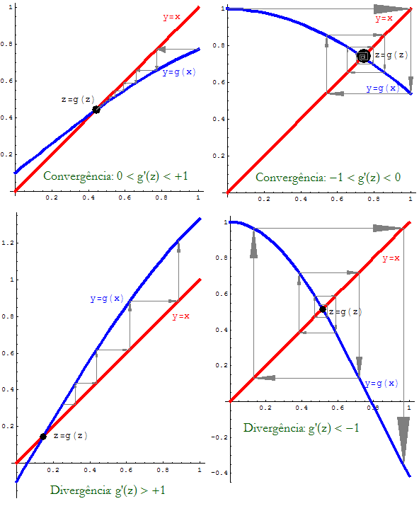Figura 1: Fixed Point Method − different cases. Convergence situations are presented in the plots above (monotone convergence − on the left, alternate convergence − on the right). The fixed point acts like an iteration atractor. On the other hand, in the two plots below the fixed point acts like an iteration repulsor. Even if we start near the fixed point the iterations diverge from that value.

Definition: We say that g is a lipschitzian function in [a, b] if there exists L > 0 such that : | g(x) − g(y) | < L | x − y | , ∀ x, y ∈ [a, b] The function is called a Contraction if the Lipschitz constant is less than one, meaning L < 1.

Note that lipschitzian functions are continuous on the interval (x→ y implies immediately g(x)→ g(y)). When the function has derivatives we relate this notion to the bounds of the derivative:

Proposição: Let g ∈ C1[a, b] such that |g '(x)| ≤ L, ∀ x ∈ [a, b], then the function g is lipschitzian in that interval, and when L < 1 it is a contraction.

dem: Using Lagrange's theorem, for any x, y in [a,b], there exists ξ ∈ ]x; y[ ⊂ [a, b] such that | g(x) − g(y) | = |g'(ξ)| |x-y| ≤ L |x − y|.

With these notions we may now present a fixed point theorem (here only for an interval).

Theorem (fixed point in a bounded interval). Let g be an iterative function in [a, b] such that: g is contractive in [a, b], g is invariant in [a, b], meaning g([a, b]) ⊆ [a, b] , then g has one and only one fixed point z ∈ [a,b] ; for any x0 ∈ [a, b], the fixed point sequence defined by xn+1 = g(xn) converges to z; we have the following error estimates: (a posteriori) (i)     | en | < L | en-1 | (ii)     | en | < L/(1-L) | xn − xn-1| (a priori) (iii)     | en | < Ln | e0 | (iv)     | en | < Ln (1-L)-1 | x1 − x0 | Here L < 1 is the contractivity constant. When g∈ C1[a,b], L = maxx∈ [a,b] |g'(x)| < 1.

proof: Existence (fixed point in an interval): it may be seen as simple consequence of the intermediate value theorem. Take f(x)=g(x)-x, the invariance hypothesis implies a≤ g(a), g(b)≤ b. Therefore, f(a)f(b)≤ 0 and there exists z∈ [a,b]: f(z)=0 ⇔ z=g(z). Uniqueness (fixed point in an interval) Suppose z,w∈ [a,b] both fixed points, z=g(z) and w=g(w). Using the contraction hypothesis |z − w| = |g(z) − g(w)| ≤ L |z − w| ⇔ (1-L)|z − w|≤ 0 and as L < 1 temos |z − w|≤ 0 that is z = w. Convergence and estimates: Using the contraction hypothesis, |en|=|z − xn| = |g(z)-g(xn-1)| ≤ L |z-xn-1| = L |en-1| we obtain the first estimate that, applied repeatedly, gives (iii) |en| ≤ Ln |e0|. As L < 1 this estimate implies |en|→ 0 (note that |e0|≤ |a-b|), and we conclude the convergence. Finally (ii) results from |en|≤ L|en-1| = L|z − xn + xn − xn-1| ≤ L|en| + L|xn − xn-1| thus (1 − L)|en| ≤ L|xn − xn-1| implies (ii). Also, (ii) implies |e1| ≤ L/(1 − L) |x1 − x0| considering n=1, and (iv) results from |en| ≤ Ln-1 |e1|.

Proposição: Under the hypothesis of the fixed point theorem, we have: (a) If 0 < g'(x) < 1, ∀ x ∈ [a, b] then we have monotone convergence (all iterations are on the same side: xn > z or xn < z) (b) If -1 < g'(x) < 0, ∀ x ∈ [a, b] then we have alternate convergence (iterations change side at each step: xnxn+1 < 0)

dem: As en = g(z) − g(xn-1) = g '(ξn) en-1 and as the sign of g' is constant, from the hypothesis, we have sign(en ) = sign( g '(ξn) ) sign(en-1 ) and obtain in case (a): sign(en ) = + sign(en-1 ) = ... = sign(e0 ), in case (b): sign(en ) = − sign(en-1 ) = ... = (-1)n sign(e0 ).

Remark: When alternate convergence is ensured, we have z∈ [xn-1; xn]. This allows to define new intervals where we have the fixed point, and we may update the value of L. For instance, assuming that -1 < g' < 0 and it is monotone, after p iterations we define a new Lp = max { -g '(xp-1); -g'(xp) }   obtaining the following estimates with these new values. A possibility for an updated a priori estimate will be |ep+k| ≤ (Lp)k | xp-1 − xp |

Example: A method to solve quadratic equations x2+bx-a=0 consists in establishing the equivalence (for x≠ -b) x2+bx-a=0 ⇔ x(x+b) = a ⇔ x = a/(x+b) where the iterative function is g(x)=c/(x+1). This leads to a sequence known as continued fraction xn+1 = a/(b+xn) = a/(b + a/(b + a/(b + ...))) that also allows to approximate square roots with fractions, in an optimal way (taking into account the size of the values). For instance, for a= b= 1, starting with x0=1 we get x1=1/2, x2=2/3, ..., x6=13/21, ..., x13=377/610, x14=610/987, ... and the last value x14 = 610/987 = 0.6180344… is a simple fraction, giving a good approximation of the exact value z=-1+√ 5=0.6180339887… We may check that in the interval I=[1/2, 1] the fixed point theorem hypothesis are verified: contractivity: g'(x)=-(1+x)-2 is increasing (g'' > 0) and it is negative, therefore L = maxx ∈ I |g'(x)|= max{ -g'(1/2), -g'(1) } = max{ 4/9, 1/4} = 4/9 < 1 invariance: g is decreasing (g' < 0 ) and we have g(1/2) = 2/3 ∈ [1/2,1], g(1) = 1/2 ∈ [1/2,1] This justifies the convergence, which is alternate (g' < 0), implying that z∈ [377/610, 610/987] and furthermore, using the a posteriori estimates (i) and (ii) we have |e14| ≤ L/(1-L) |x14-x13| = 4/5×0.166…10-5 < 0.133×10-5 As g' is increasing and negative, considering a reduced interval L14= max {|g'(x13)|, |g'(x14)| } = 0.381966… and we have a precise estimate for the following iterations |e14+k|≤ 0.382k (0.133×10-5)

Theorem (Non convergence or "divergence"): Let g∈ C1(Vz) where Vz is a neighborhood of the fixed point z. If | g '(z) | > 1, the fixed point sequence never converges to z, except if xp=z (at some step p).

proof: We saw, using Lagrange's theorem: en+1 = g '(ξn) en with ξn∈ [xn;z] ⊂ Vz considering xn sufficiently close to z. Since | g '(z) | > 1, then in the neighborhood we have also | g '(ξ) | > 1, (because g∈ C1(Vz)). Since en ≠ 0 (as xn≠ z) |en+1| = |g '(ξn)| |en| > |en| and the error increases, making convergence impossible.

This is a local result, that allows to conclude non convergence as long as we show that the derivate (in modulus) is greater than 1, in an interval that contains the fixed point. As a counterpart we may establish a local convergence result. This result is slightly different from the fixed point theorem, as it does not demand invariance, but we need have an a priori location of the fixed point, as the initial iterate must be sufficiently close to it.

Theorem (Local convergence): Let g∈ C1(Vz) where Vz is a neighborhood of the fixed point z. If | g '(z) | < 1, the fixed point sequence converges to z, when x0 is sufficiently close to z.

proof: This result may be reduced to the fixed point theorem considering Wz = {x: |x − z| ≤ ε} with ε small enough to have a contraction, |g'(x)| < 1, ∀ x∈ Wz⊂ Vz , as |g'(z)| < 1 and g∈ C1(Vz). Therefore, if x∈ Wz we have |g(x) − z| = |g '(ξ)| |x − z | ≤ ε ⇐ g(x)∈ Wz and invariance is shown. Thus, we conclude the convergence by the fixed point theorem, as long as x0∈ Wz, meaning, for initial iterates sufficiently close to z.

Within convergence cases, there are sequences that converge more rapidly than others. Thus, it is appropriate to distinguish the order of convergence.

Definition Let (xn) be a sequence that converges to z. We say that (xn) has order of convergence p with asymptotic coefficient Kp ≠ 0 if the following limit exists limn→∞   |en+1| |en|p = Kp ≠ 0

Note that K1≤ 1 because if K1 > 1 no convergence occurs: |en+1| > |en| (the error increases).   We distinguish 3 main classes of convergence: Superlinear (or Exponential): when p>1 (or p=1 and K1 = 0). Linear: p=1 and 0 < K1 < 1 Sublinear (or Logarithmic): p=1 and K1 = 1 There are other names as quadratic convergence when p=2, cubic convergence when p=3 (these convergence orders are different from the ones given in the context of approximation, as in quadrature rules). Note that if the limit is Kp=0 this means that the convergence is at least of order p, but then one should look for an higher p, to obtain the correct order of convergence.

Examples: We present some examples that are not necessarily connected to the fixed point method. (i) Let xn = αn with 0 < α < 1. This sequence converges to z=0, and we have K1 = limn→∞   |en+1| |en| = limn→∞   |αn+1| |αn| = α ≠ 0 this means a linear convergence with K1 = α. (ii) Let xn = αβ^n with 0 < α < 1 < β. [note that xn = α^(β^n) is different from (α^β)^n = α^(β n) ] This sequence also converges to z=0, but we have K1 = limn→∞   |en+1| |en| = limn→∞   |αβ^(n+1)| |αβ^n| = limn→∞   |(αβ^n)β| |αβ^n| = limn→∞ (αβ^n)β-1 = 0 and we have superlinear convergence (K1 = 0). To identify the exact order, we check Kβ = limn→∞   |en+1| |en|β = limn→∞ (αβ^n)β-β = 1 ≠ 0 concluding that the order of convergence is β > 1. (iii) Finally a logarithmic convergence result. Take xn = n-b with b>0, that converges to z=0. As, K1 = limn→∞   |en+1| |en| = limn→∞   |(n+1)-b| |n-b| = limn→∞ (1+1/n)-b = 1-b = 1 we conclude the sublinear convergence.

Theorem (Fixed point method − order of convergence): Let g∈ Cp(Vz) where Vz is a neighborhood of the fixed point z. If g(p)(z)≠ 0, e g'(z) = ... = g(p-1)(z) = 0, then the (local) order of convergence of the fixed point sequence is p, and the asymptotic coefficient is given by Kp = |g(p)(z)| / p! (note that for p=1, this implies K1 < 1 to have local convergence).

proof: The local convergence was ensured in the previous theorem for K1 = |g'(z)| < 1. Using the Taylor expansion with Lagrange remainder g(xn) = g(z) + g(p)(ξn)/p! (-en)p, com ξn ∈ [xn;z] because g'(z) = ... = g(p-1)(z) = 0. On the other hand, g(xn)=xn+1 and z = g(z) means - en+1 = g(p)(ξn)/p!   (-en)p, Thus, substituting in Kp = limn→∞   |en+1| |en|p = limn→∞ |g(p)(ξn)|/p! = |g(p)(z)| / p! ≠ 0 we conclude that the order of convergence is p.

Remark: (i) It is an immediate consequence of the definition of order of convergence that if a method has order of convergence p > 1, a method grouping two iterations will have order of convergence 2p. Therefore, it is a qualitative difference to obtain superlinear convergence, and it is a secondary issue to obtain higher orders of convergence (despite some emphasis in the usual literature). Furthermore, if the convergence is just linear, a new method grouping two iterations, will just reduce the asymptotic coefficient to one half. Thus, the order of convergence plays a similar role to superlinear methods, as the role of the asymptotic coefficient in linear convergent methods. (ii) Another possibility to define order of convergence p, consists in having a constant Kp > 0 such that |en+1| ≤ Kp |en|p   (n sufficiently large) (when p=1 we must have K1< 1), and it is not necessary that the limit exists. Furthermore, knowing the order of convergence, we may establish a relation between the difference of iterations and the absolute error: |en| =   |xn+1 − xn| |1 − en+1/en| ≤   |xn+1 − xn| 1 − Kp |en|p-1 as long as Kp |en|p-1 < 1. We conclude that |en| ≤   Kp |en-1|p-1 1 − Kp |en-1|p-1 |xn − xn-1| ... this expression was already known for p=1 (the condition K1 < 1 is necessary for the linear convergence).   Based on the difference of iterations we may define a stopping criteria, noticing that |en| ≤   Ln 1 − Ln |xn − xn-1|, when Ln = Kp |en-1|p-1 < 1 (this will happen for some n as en → 0).

Newton Method

The previous theorem allows to conclude superlinear convergence if the iterative function as a null derivative in the fixed point. Thus we are led to search methods with this property.   When f '(x) ≠ 0 we may establish an equivalence f(x) = 0 ⇔ x = x − f(x)/f '(x) and define the iterative function g(x) = x − f(x)/f '(x). For the root z, as f(z)=0, we get g'(x) = f(x) f ''(x)/(f '(x))2   ⇒   g'(z) = 0 Therefore, according to the previous theorem, in this case we have at least quadratic convergence (it might be cubic, if f '(z) ≠ 0, f ''(z) = 0).   Newton Method consists in applying the fixed point method to this g, meaning Given an initial iterate x0 ; Repeat   xn+1 = xn − f(xn )/f '(xn ) . and as we saw, excluding the case f '(z)=0, we ensure at least quadratic convergence.   Remarks: (1) Newton Method has also a geometrical interpretation that is related to its original deduction (this method is also called Newton-Raphson Method, or Tangent Method) as presented in Fig. 2. 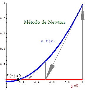Figura 2: Iterations in Newton Method. Starting with x0=1, the new point x1 results from the intersection of the tangent line with the axis y=0, and so on.   The geometrical deduction consists in using the tangent line y = f(xn) + f '(xn)(x-xn) as an approximation of f in xn (it is the first order approximation in Taylor's expansion). Deducing the solution x such that y=0 we obtain the same expression 0 = f(xn) + f '(xn)(x-xn) ⇔ x = xn − f(xn)/f '(xn) this solution x is the new approximation xn+1.   (2) We may be led to deduce higher approximations, increasing the order of the Taylor expansion. This leads to a higher order of convergence but also to more complex expressions, that are computationally less efficient than grouping iterations (see previous remarks). In fact n iterations with Newton Method are usually more efficient than a single iteration with some other methods of order 2n.

Examples: We present some examples that show the performance of Newton Method. (i) Calculate z= p√ a using only arithmetical operations. Note that here z is the solution of f(x) = xp − a = 0. According to the local convergence theorem, we take a sufficiently close x0, and the method resumes to xn+1 = xn − (xnp-a)/(p xnp-1) = xn(1-1/p) + (a/p) xn1-p it is even simpler to extract square roots (p=2) xn+1 = xn/2 + a/(2 xn) (this is useful in binary FP systems, as the divisions/products by 2 are trivial). (ii) Consider for instance the calculation of z= 3√ 6: x0 = 2, x1 = 11/6, x2 = 1.817263…, x3 = 1.81712060…, x4 = 1.817120592832139… in this 4th iterate all the presented digits are correct. (iii) Recovering the continued fraction example, the application of Newton Method to f(x)=x2+bx-a=0 leads to calculations that involve also simple fractions xn+1 = xn − ((xn+b)xn-a)/(2xn+b) = (xn2+a)/(2xn+b) obtaining for x0=1 x1=2/3, x2=13/21, x3=610/987, x4=1346269/2178309, ... Note that these are the values that we also obtained in the continued fraction, but in a much faster way (here the 2nd iteration is the 6th iteration in the continued fraction, the 3rd is the previous 14th, and the 4th is the previous 30th). The fraction x4 presents an error below 10-13.

Again, we are also interested in establishing sufficient conditions that ensure a convergence that is not only local (for a "sufficiently close initial iterate"), but that is valid for a set of initial iterates in an interval.

Theorem (Convergence of Newton Method − sufficient conditions for an interval): Let f∈ C2[a,b] such that in the interval (x ∈ [a, b]) (1) f(a) f(b) ≤ 0 ; (2) f ' (x) > 0 ou f ' (x) < 0 ; (3) f '' (x) ≥ 0 ou f '' (x) ≤ 0 ; Then Newton Method has at least quadratic convergence to the unique solution z ∈ [a,b], initializing the method: (a) with x0∈ [a,b] : f(x0) f ''(x) ≥ 0 (b) for any x0∈ [a,b] if |f(a)/f '(a)|, |f(b)/f '(b)| ≤ |b − a|

proof: A non constructive proof is simple but not relevant here, we prefer to discuss the conditions: Note that conditions 1) and 2) imply existence and uniqueness. Condition 3) is important such that the convexity does not change, leading to a cyclic, non convergent situation: − For instance, if f(x) = x3 − 5 x, in [-1,1] there a single solution (z=0) and conditions 1) and 2) are verified, but not the condition 3), since f ''(x)=6x changes sign in [-1,1]. As a consequence we see that x0 = 1, x1 = 1 − (1-5)/(3-5) = -1, x2 = 1, ..., xk = (-1)k, and the sequence defined by Newton Method does not converge! Finally, note that condition (a) is always verified in one of the interval limits, but to ensure convergence for x0 at any point of the interval, the condition (b) guarantees that iterates starting do not fall off the interval... for instance, if x0=a x1 = a − f(a)/f '(a) ⇐ |x1 − a| = |f(a)/f '(a)| ≤ |b − a| Finally, the convergence is monotone for initial iterates verifying (a). Condition (b) has only to be verified for the limit that does not verify (a) then having x1 as a starting point verifying (a) and monotone convergence for the next iterations.

Theorem (Newton Method − Error Estimates): Let f∈ C2[a,b] and assume the previous quadratic convergence conditions. We have the following error formula: ∃ ξ ∈ [xn; z] :     en+1 = −   f ''(ξ) 2 f '(xn) (en)2 this leads to the asymptotic coefficient K2 =   |f ''(z)| 2 |f '(z)| and to the estimates (a posteriori) |en| ≤   maxx∈ [a,b] |f ''(x)| 2 |f '(xn-1)| |en-1|2 (a priori) M |en| ≤ (M|e0|)2^n where M =   maxx∈ [a,b] |f ''(x)| 2 minx∈ [a,b]|f '(x)|

proof: − The Error Formula results from the Taylor expansion 0 = f(z) = f(xn) + f '(xn)(z-xn) + ½f ''(ξn)(-en)2 dividing by f '(xn)≠ 0 we obtain 0 = f(xn)/f '(xn) + z − xn + ½f ''(ξn)/f '(xn)(en)2 and as f(xn)/f '(xn) − xn = -xn+1 we get, 0 = z − xn+1 + ½f ''(ξn)/f '(xn)(en)2 with ξ ∈ [xn; z] and xn → z. We get K2 dividing |en+1| by |en|2. Finally − the first estimate is immediate, since ξ ∈ [xn; z]⊂ [a,b]. − the second estimate is also immediate, as M |en| ≤ (M|en-1|)2 applying it repeatedly.

Remarks:     (i) When f '(z)=0 we are in the situation of a double root (at least), and Newton Method loses quadratic convergence, being possible a slight change to recover quadratic convergence (e.g. [CA]).     (ii) When f ''(z)=0 (and f'(z) ≠ 0) we obtain a cubic convergence.     (iii) As an empirical rule quadratic convergence means doubling the number of significant digits in each iterate (... cubic convergence means the triple). This means that near the root, double precision exact value is achieved in less than 4 or 5 iterations, being more important to get there in the first place.     (iv) We stress this point, as it follows from the error estimates that to have an acceptable a priori estimate the value M|e0| should be less than 1, and this means that the initial iterate should not be far from the solution (moreover if |f '| is small or |f ''| is large).

Example: Consider f(x)= e-x − log(x) = 0, that verifies in the interval [1,2]: 1) f(1) = e-1 > 0,   f(2) = e-2-log(2) < 0; 2) f '(x) = -e-x-1/x < 0 (for x∈ [1,2]) 3) f ''(x) = e-x+1/x2 > 0 (for x∈ [1,2]) the sufficient conditions for Newton Method convergence are verified, at least for initial iterates such that f(x0)>0 [conclusion (a) from the Theorem], as it is the case for x0=1. Since |f(1)/f '(1)| = 0.2689… , |f(2)/f '(2)| = 0.87798… < |2-1| = 1, following conclusion (b), we have convergence given any x0∈ [1,2]. Starting with x0=1 we get x1=1.2689…, x2=1.309108…, x3=1.3097993887… as |f(x3)|≤ 2.04× 10-7 and min[1,2]|f '|=|f '(2)| > 0.635, the general a posteriori estimate gives us |e3|≤ 2.04× 10-7 / 0.635 < 3.21× 10-7. and we see that x3 already presents 7 correct digits. Using this information we may improve the next estimates. The interval is now small enough to consider M≈ K2 ≈ 0.413, therefore 0.412|ek+3| ≤ (M|e3|)2^k ≤ (1.325× 10-7)2^k meaning that x5=1.30979958580415… presents an error bound |e5|≤ 0.412-1(1.325× 10-7)4 < 10-27 being completely useless other double precision iterations, as only the rounding error will remain.

Secant Method

The Secant Method is a variant of Newton Method, as it avoids the calculation of derivatives substituting them by a finite difference approximation (that in the limit coincides with derivative itself).   Like the Newton Method, the Secant Method may be deduced in a geometrical way, substituting the tangent line by a secant line. Given two points xn-1 and xn we define the "secant line" that crosses the image points: y = f(xn) +   f(xn) − f(xn-1) xn − xn-1 (x − xn) the derivative is now substituted by the finite difference. In a similar way, solving for y=0 we get x = xn −   xn − xn-1 f(xn) − f(xn-1) f(xn) and this will be the new approximation value xn+1.   Resuming, Secant Method consists in Defining two initial iterates x-1 e x0. Repeat xn+1 = xn −   xn − xn-1 f(xn) − f(xn-1) f(xn) Remark: Note that in each iteration we do not need to calculate two times the function f, as the value f(xn-1) is to be stored from the previous iteration. This way the method is computationally more efficient than Newton Method (in most cases), as it does not demand an updated calculation of the derivative at each step.   Error Formula (Secant Method) It is possible to establish the following formula (check details in [KA]) ∃ ξn, ηn ∈ [xn-1; xn; z] : en+1 = −   f ''(ξn) 2 f '(ηn) en en-1 allowing the error estimate |en+1| ≤   max |f ''(x)| 2 min |f '(x)| |en| |en-1| The convergence is again superlinear (but not quadratic) when f '(z) ≠ 0, since limn→∞   |en+1| |en| = limn→∞   |f ''(ξn)| 2 |f '(ηn)| |en-1| =   |f ''(z)| 2 |f '(z)| limn→∞ |en-1| = 0 since |en|→ 0 (assuming convergence). It may be shown (e.g. [KA]) that if f '(z) ≠ 0 the order of convergence of Secant Method is p=(1+√ 5)/2 = 1.618… the golden number.   NOTE: In fact, taking yn = log|en| and applying logarithms to the formula, we establish (hand waive argument) yn+1 ≈ C + yn + yn-1 a Fibonacci sequence, and from the ratio yn+1/yn → p we get log|en+1|≈ p log|en|, which is a simple justification for this golden value of p.

Theorem (Convergence of the Secant Method − sufficient conditions in an interval) Let f ∈ C2[a,b]. In the hypothesis (1), (2), (3), of the similar theorem for Newton Method, Secant method has a superlinear order of convergence p = 1.618…, initializing (a) with x-1, x0 ∈ [a,b] : f(x-1)f ''(x) ≥ 0 , f(x0)f ''(x) ≥ 0 (b) with any x-1, x0 ∈ [a,b]   if   |f(a)/f '(a)|, |f(b)/f '(b)| ≤ |b − a|

Example: Consider again f(x)= e-x-log(x) = 0 the conditions (1), (2), (3) were already verified in [1,2]. As the condition (b) was also verified, we may use any pair of initial iterates to obtain with the Secant Method a sequence with superlinear convergence. Starting with x-1=1, x0=1.5, we get x5=1.309799585804… com |e5|≤ |f(x5)|/0.635 < 2× 10-13 (using the general a posteriori estimate) being enough to calculate another iteration to have the exact full digits in double precision.

Final Remarks and References

It should be noticed that there several other popular numerical methods for root finding, some of them combine several of the previous methods. For instance Brent's Method uses both Bisection and the Secant methods (along with inverse quadratic interpolation). For complex root finding, Fixed-point, Newton or Secant methods have straightforward generalizations. There is a sort of generalization for the Bisection method, the Lehmer-Schur algorithm, that consists in calculating the winding number along 4 smaller squares, at each step. We will some of these generalizations in the next chapters. [CA] C. J. S. Alves, Fundamentos de Análise Numérica (I), Secção de Folhas AEIST (2002). [KA] K. Atkinson: An Introduction to Numerical Analysis, Wiley (1989)